Tutorial
Splitter Optimization
Let’s have a look at the code in examples/splitter/splitter_opt.py
""" Copyright chriskeraly
    Copyright (c) 2019 Lumerical Inc. """

######## IMPORTS ########
# General purpose imports
import os
import numpy as np
import scipy as sp

# Optimization specific imports
from lumopt.utilities.wavelengths import Wavelengths
from lumopt.geometries.polygon import FunctionDefinedPolygon
from lumopt.figures_of_merit.modematch import ModeMatch
from lumopt.optimizers.generic_optimizers import ScipyOptimizers
from lumopt.optimization import Optimization

######## DEFINE BASE SIMULATION ########
base_script = os.path.join(os.path.dirname(__file__), 'splitter_base_TE_modematch.lsf')

######## DEFINE SPECTRAL RANGE #########
# Global wavelength/frequency range for all the simulations
wavelengths = Wavelengths(start = 1300e-9, stop = 1800e-9, points = 21)

######## DEFINE OPTIMIZABLE GEOMETRY ########
# The class FunctionDefinedPolygon needs a parameterized Polygon (with points ordered
# in a counter-clockwise direction). Here the geometry is defined by 10 parameters defining
# the knots of a spline, and the resulting Polygon has 200 edges, making it quite smooth.
initial_points_x = np.linspace(-1.0e-6, 1.0e-6, 10)
initial_points_y = np.linspace(0.25e-6, 0.6e-6, initial_points_x.size)
def taper_splitter(params = initial_points_y):
    ''' Defines a taper where the paramaters are the y coordinates of the nodes of a cubic spline. '''
    points_x = np.concatenate(([initial_points_x.min() - 0.01e-6], initial_points_x, [initial_points_x.max() + 0.01e-6]))
    points_y = np.concatenate(([initial_points_y.min()], params, [initial_points_y.max()]))
    n_interpolation_points = 100
    polygon_points_x = np.linspace(min(points_x), max(points_x), n_interpolation_points)
    interpolator = sp.interpolate.interp1d(points_x, points_y, kind = 'cubic')
    polygon_points_y = interpolator(polygon_points_x)
    polygon_points_up = [(x, y) for x, y in zip(polygon_points_x, polygon_points_y)]
    polygon_points_down = [(x, -y) for x, y in zip(polygon_points_x, polygon_points_y)]
    polygon_points = np.array(polygon_points_up[::-1] + polygon_points_down)
    return polygon_points

# The geometry will pass on the bounds and initial parameters to the optimizer.
bounds = [(0.2e-6, 0.8e-6)] * initial_points_y.size
# The permittivity of the material making the optimizable geometry and the permittivity of the material surrounding
# it must be defined. Since this is a 2D simulation, the depth has no importance. The edge precision defines the
# discretization of the edges forming the optimizable polygon. It should be set such there are at least a few points
# per mesh cell. An effective index of 2.8 is user to simulate a 2D slab of 220 nm thickness.
geometry = FunctionDefinedPolygon(func = taper_splitter, initial_params = initial_points_y, bounds = bounds, z = 0.0, depth = 220e-9, eps_out = 1.44 ** 2, eps_in = 2.8 ** 2, edge_precision = 5, dx = 1e-9)

######## DEFINE FIGURE OF MERIT ########
# The base simulation script defines a field monitor named 'fom' at the point where we want to modematch to the 3rd mode (fundamental TE mode).
fom = ModeMatch(monitor_name = 'fom', mode_number = 2, direction = 'Forward', multi_freq_src = True, target_T_fwd = lambda wl: np.ones(wl.size), norm_p = 1)

######## DEFINE OPTIMIZATION ALGORITHM ########
# This will run Scipy's implementation of the L-BFGS-B algoithm for at least 40 iterations. Since the variables are on the
# order of 1e-6, thery are scale up to be on the order of 1.
optimizer = ScipyOptimizers(max_iter = 30, method = 'L-BFGS-B', scaling_factor = 1e6, pgtol = 1e-5)

######## PUT EVERYTHING TOGETHER ########
opt = Optimization(base_script = base_script, wavelengths = wavelengths, fom = fom, geometry = geometry, optimizer = optimizer, hide_fdtd_cad = False, use_deps = True)

######## RUN THE OPTIMIZER ########
opt.run()
Optimization Philosophy
- The optimization setup works as such:
- The user must provide a Lumerical script that serves as the basis of the optimization. It has everything required to build the problem except for the optimizable geometry, which is defined later in the python script and added in the simulation by the optimization itself.
- The user then defines in python, using the classes of LumOpt:
- An optimizable geometry
- A Figure of Merit
- An Optimization algorithm
Lumerical Setup Script
Here is the setup script examples/Ysplitter/splitter_base_TE_modematch.lsf used in this example:
# Copyright chriskeraly
# Copyright (c) 2019 Lumerical Inc.

switchtolayout;
selectall;
delete;

## SIM PARAMS
size_x=3e-6;
size_y=3e-6;
mesh_x=20e-9;
mesh_y=20e-9;
finer_mesh_size=2.5e-6;
mesh_accuracy=2;

## GEOMETRY

#INPUT WAVEGUIDE
addrect;
set('name','input wg');
set('x span',3e-6);
set('y span',0.5e-6);
set('z span',220e-9);
set('y',0);
set('x',-2.5e-6);
set('index',2.8);

#OUTPUT WAVEGUIDES
addrect;
set('name','output wg top');
set('x span',3e-6);
set('y span',0.5e-6);
set('z span',220e-9);
set('y',0.35e-6);
set('x',2.5e-6);
set('index',2.8);

addrect;
set('name','output wg bottom');
set('x span',3e-6);
set('y span',0.5e-6);
set('z span',220e-9);
set('y',-0.35e-6);
set('x',2.5e-6);
set('index',2.8);

## SOURCE
addmode;
set('direction','Forward');
set('injection axis','x-axis');
#set('polarization angle',0);
set('y',0.0);
set('y span',size_y);
set('x',-1.25e-6);
set('override global source settings',false);
set('mode selection','fundamental TE mode');

## FDTD
addfdtd;
set('dimension','2D');
set('background index',1.44);
set('mesh accuracy',mesh_accuracy);
set('x',0.0);
set('x span',size_x);
set('y',0.0);
set('y span',size_y);
set('force symmetric y mesh',true);
set('y min bc','Anti-Symmetric');
set('pml layers',12);

## MESH IN OPTIMIZABLE REGION
addmesh;
set('x',0);
set('x span',finer_mesh_size+2.0*mesh_x);
set('y',0);
set('y span',finer_mesh_size);
set('dx',mesh_x);
set('dy',mesh_y);

## OPTIMIZATION FIELDS MONITOR IN OPTIMIZABLE REGION
addpower;
set('name','opt_fields');
set('monitor type','2D Z-normal');
set('x',0);
set('x span',finer_mesh_size);
set('y',0);
set('y span',finer_mesh_size);

## FOM FIELDS
addpower;
set('name','fom');
set('monitor type','2D X-normal');
set('x',finer_mesh_size/2.0);
set('y',0.0);
set('y span',size_y);
If the setup script is run in Lumerical FDTD (or alternatively replace opt.run() with opt.make_base_sim() in the previous code snippet, here is a screenshot of what is built:
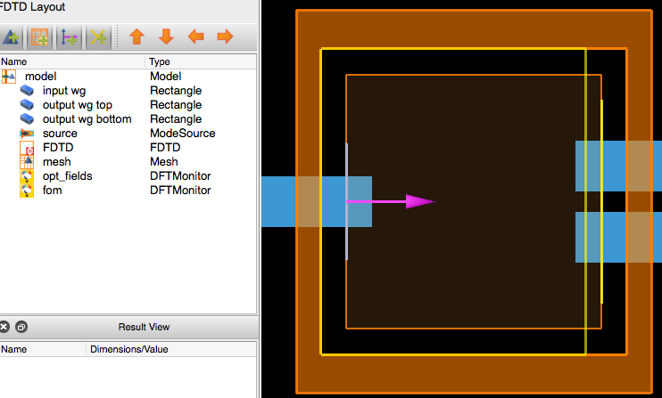
As one can see everything but the optimizable geometry is present. There are some additional requirements to this base simulation however, beyond the strict minimum to perform the simulation.
Base Simulation Requirements:
SOURCES:
Sources MUST have ‘source’ in their name. This is because to run the adjoint simulation, all the classic forward simulation sources will have to be deleted. The easiest way to do this is to identify by their name. IF YOU HAVE A SOURCE WITHOUT ‘source’, IN ITS NAME YOUR OPTIMIZATION WILL MOST LIKELY FAIL.
OPTIMIZATION FIELD MONITOR:
A field Monitor named ‘opt_fields’ must cover the entire region where your optimizable geometry is succeptible to go. This is because the fields in your optimizable geometry must be known in order to calculate the shape derivatives. Make sure that even once the optimization gets going, your geometry will not go beyond this box. If it does the optimization will crash. Be particularly carefull with splines, which can sometimes shoot well beyond their knots.
MESH:
In the same way as the optimization field monitor above, a mesh refinement region should be placed over the region where the geometry is succeptible to go. This is to ensure that the mesh does not change during the optimization, which would also cause the optimization to crash.
Co-optimization
The + operator can be used between two optimization objects that use the same parameters. This is for the moment the only way to do multi-wavelength optimization for example.
An example of this can be seen in examples/Ysplitter/robust_coupler.py where a the performance of a coupler is optimized for robustness: the figure of merit is the sum of the figures of merit for the nominal geometry, and a geometry with a 25nm extra bias.
""" Copyright chriskeraly
    Copyright (c) 2019 Lumerical Inc. """

######## IMPORTS ########
# General purpose imports
import os
import numpy as np
import scipy as sp

from lumopt.utilities.wavelengths import Wavelengths
from lumopt.geometries.polygon import FunctionDefinedPolygon
from lumopt.figures_of_merit.modematch import ModeMatch
from lumopt.optimizers.generic_optimizers import ScipyOptimizers
from lumopt.optimization import Optimization

######## DEFINE SPECTRAL RANGE #########
wavelengths = Wavelengths(start = 1550e-9, stop = 1550e-9, points = 1)

######## DEFINE BASE SIMULATION ########
# Use the same script for both simulations, but it's just to keep the example simple. You could use two.
script_1 = os.path.join(os.path.dirname(__file__), 'splitter_base_TE_modematch.lsf')
script_2 = os.path.join(os.path.dirname(__file__), 'splitter_base_TE_modematch_25nmoffset.lsf')

######## DEFINE OPTIMIZABLE GEOMETRY ########
## Here the two splitters just have a 25nm offset from each other, so that the result is robust
initial_points_x = np.linspace(-1.0e-6, 1.0e-6, 10)
initial_points_y = np.linspace(0.25e-6, 0.6e-6, initial_points_x.size)
def taper_splitter_1(params = initial_points_y):
    points_x = np.concatenate(([initial_points_x.min() - 0.01e-6], initial_points_x, [initial_points_x.max() + 0.01e-6]))
    points_y = np.concatenate(([initial_points_y.min()], params, [initial_points_y.max()]))
    n_interpolation_points = 100
    polygon_points_x = np.linspace(min(points_x), max(points_x), n_interpolation_points)
    interpolator = sp.interpolate.interp1d(points_x, points_y, kind = 'cubic')
    polygon_points_y = interpolator(polygon_points_x)
    polygon_points_up = [(x, y) for x, y in zip(polygon_points_x, polygon_points_y)]
    polygon_points_down = [(x, -y) for x, y in zip(polygon_points_x, polygon_points_y)]
    polygon_points = np.array(polygon_points_up[::-1] + polygon_points_down)
    return polygon_points

dy = 25.0e-9
def taper_splitter_2(params = initial_points_y + dy):
    points_x = np.concatenate(([initial_points_x.min() - 0.01e-6], initial_points_x, [initial_points_x.max() + 0.01e-6]))
    points_y = np.concatenate(([initial_points_y.min() + dy], params, [initial_points_y.max() + dy]))
    n_interpolation_points = 100
    polygon_points_x = np.linspace(min(points_x), max(points_x), n_interpolation_points)
    interpolator = sp.interpolate.interp1d(points_x, points_y, kind = 'cubic')
    polygon_points_y = interpolator(polygon_points_x)
    polygon_points_up = [(x, y) for x, y in zip(polygon_points_x, polygon_points_y)]
    polygon_points_down = [(x, -y) for x, y in zip(polygon_points_x, polygon_points_y)]
    polygon_points = np.array(polygon_points_up[::-1] + polygon_points_down)
    return polygon_points

bounds = [(0.2e-6, 0.9e-6)] * initial_points_y.size
# guess from splitter_opt_2D.py optimization
initial_params = np.array([2.44788514e-07, 2.65915795e-07, 2.68748023e-07, 4.42233947e-07, 6.61232152e-07, 6.47561406e-07, 6.91473099e-07, 6.17511522e-07, 6.70669074e-07, 5.86141086e-07])
geometry_1 = FunctionDefinedPolygon(func = taper_splitter_1, initial_params = initial_points_y, bounds = bounds, z = 0.0, depth = 220e-9, eps_out = 1.44 ** 2, eps_in = 2.8 ** 2, edge_precision = 5, dx = 0.1e-9)
geometry_2 = FunctionDefinedPolygon(func = taper_splitter_2, initial_params = initial_points_y + dy, bounds = bounds, z = 0.0, depth = 220e-9, eps_out = 1.44 ** 2, eps_in = 2.8 ** 2, edge_precision = 5, dx = 0.1e-9)

######## DEFINE FIGURE OF MERIT ########
# Although we are optimizing for the same thing, two separate fom objects must be create
fom_1 = ModeMatch(monitor_name = 'fom', mode_number = 3, direction = 'Forward', multi_freq_src = False, target_T_fwd = lambda wl: np.ones(wl.size), norm_p = 1)
fom_2 = ModeMatch(monitor_name = 'fom', mode_number = 3, direction = 'Forward', multi_freq_src = False, target_T_fwd = lambda wl: np.ones(wl.size), norm_p = 1)

######## DEFINE OPTIMIZATION ALGORITHM ########
#For the optimizer, they should all be set the same, but different objects. Eventually this will be improved
optimizer_1 = ScipyOptimizers(max_iter = 40, method = 'L-BFGS-B', scaling_factor = 1e6, pgtol = 1e-9)
optimizer_2 = ScipyOptimizers(max_iter = 40, method = 'L-BFGS-B', scaling_factor = 1e6, pgtol = 1e-9)

######## PUT EVERYTHING TOGETHER ########
opt_1 = Optimization(base_script = script_1, wavelengths = wavelengths, fom = fom_1, geometry = geometry_1, optimizer = optimizer_1, hide_fdtd_cad = False, use_deps = True)
opt_2 = Optimization(base_script = script_2, wavelengths = wavelengths, fom = fom_2, geometry = geometry_2, optimizer = optimizer_2, hide_fdtd_cad = False, use_deps = True)
opt = opt_1 + opt_2

######## RUN THE OPTIMIZER ########
opt.run()
which yields: